Currently trying out a different aesthetic for my website for the new year.
Blog
-

Building a RESTful API for Sentiment Analysis
This is a project on creating an NLP Model deployment using Python, Flask, and Postman.
Project Overview
This project is a sentiment analysis tool. It classifies text (movie reviews) as positive or negative. This classification is done using natural language processing (NLP) techniques. It includes:
– Text Pre-processing
– Machine Learning Model Training
– Flask API Development
This project allows users to enter a sentence. They can receive a prediction of its sentiment, either positive or negative, via an API endpoint.
Dataset
Dataset Name: UCI Sentiment Labelled Sentences
Description: This dataset contains labeled sentences categorized as positive (1) or negative (0).
Source: UCI Machine Learning Repository
Data Format: .txt file with sentences and labels.
Project Workflow
The project consists of several main steps:
1. Data Loading: Loading and reading the .txt file format of the dataset.
2. Data Pre-processing: Cleaning and tokenizing text, removing stopwords.
3. Feature Extraction: Converting text data into numerical features using TF-IDF Vectorizer.
4. Model Training: Training a logistic regression model on the pre-processed data.
5. Model Evaluation: Evaluating the model on test data and assessing its performance.
6. API Development: Creating an API with Flask to expose the model as a service.
Model Training and Evaluation
Algorithm Used: Logistic Regression
Feature Engineering: TF-IDF Vectorizer
Evaluation Metrics:
– Accuracy: Measured to determine the overall performance of the model.
– Confusion Matrix: Visualizes the classification performance.
API Development
I created a RESTful API using Flask. It allows users to make POST requests with sentences about movie reviews. Users can then receive sentiment predictions.
Endpoint: /predict
Method: POST
Expected Input: JSON payload with a ‘sentence’ field.
{“sentence”: “I love this movie!”}
Response:
{“prediction”: 1}
Setup and Installation
Prerequisites: Python 3.7+, pip for package management
Installation Steps:
1. Clone the Repository:
git clone https://github.com/ernestog27/data-projects.git
2. Create and Activate a Virtual Environment:
python3 -m venv sentiment_env
source sentiment_env/bin/activate
3. Install Required Libraries:pip install -r requirements.txt
4. Run the Flask Application:
NLP_sentiment_analysis.py
Usage
Using Postman to Test the API:
1. Open Postman and set the request method to POST.
2. Enter the endpoint URL: http://127.0.0.1:5000/predict
3. Set Headers:
– Key: Content-Type, Value: application/json
4. Request Body: Choose ‘raw’ and JSON format, then enter:
{“sentence”: “This movie is amazing!”}
5. Send Request: Postman will return the sentiment prediction.
Results
Accuracy: The model achieved an accuracy of 75.3% on the test dataset.

Sample Predictions:
– ‘The movie was fantastic!’ -> Positive (1)
– ‘I did not enjoy the movie.’ -> Negative (0)
Confusion Matrix:

Future Improvements
Expand Dataset: Add more labeled sentences for training.
Model Optimization: Experiment with other models (e.g., SVM, neural networks) and hyper-parameter tuning.
Real-Time Updates: Retrain the model periodically with new data to improve prediction accuracy.
References:
Kotzias, D. (2015). Sentiment Labelled Sentences [Dataset]. UCI Machine Learning Repository. https://doi.org/10.24432/C57604.
Here is the link for latest python code:
And below is a snapshot of the code for illustration purposes as of November 2024.
For the latest see link above.
# Sentiment Analysis API with Flask
# Ernesto Gonzales, MSDA

import pandas as pd

# Loading the dataset
data = pd.read_csv('sentiment_env/databases/sentiment labelled sentences/imdb_labelled.txt', delimiter = '\t', header = None)
data.columns = ['Sentence', 'Label'] # Rename columns for clarity

# Data preview
print(data.head())
print(data.info())
print(data['Label'].value_counts())

# Data Cleaning and Pre-processing

import nltk
from nltk.corpus import stopwords
from nltk.tokenize import word_tokenize
import re

# Downloading necessary NLTK data

nltk.download('stopwords')
nltk.download('punkt_tab')

# Function for text cleaning

def preprocess_text(text):
    text = re.sub(r'\W', ' ', text) # Remove non-word characters
    text = text.lower() # Convert text to lowercase
    words = word_tokenize(text) # Tokenize text
    words = [word for word in words if word not in stopwords.words('english')] # Remove stopwords
    return ' '.join(words)

# Applying function to the text column

data['Cleaned_Sentence'] = data['Sentence'].apply(preprocess_text)

# Spliting data into training and testing sets

from sklearn.model_selection import train_test_split
X = data['Cleaned_Sentence']
y = data['Label']
X_train, X_test, y_train, y_test = train_test_split(X, y, test_size = 0.2, random_state = 42)

# Feature extraction

from sklearn.feature_extraction.text import TfidfVectorizer
vectorizer = TfidfVectorizer(max_features = 5000)
X_train_tdif = vectorizer.fit_transform(X_train)
X_test_tfidf = vectorizer.transform(X_test)

# Training and Evaluating model

from sklearn.linear_model import LogisticRegression

model = LogisticRegression()
model.fit(X_train_tdif, y_train)

from sklearn.metrics import accuracy_score, classification_report

y_pred = model.predict(X_test_tfidf)
print(f"Accuracy: {accuracy_score(y_test, y_pred)}")
print(classification_report(y_test,y_pred))

from sklearn.metrics import ConfusionMatrixDisplay, confusion_matrix
import matplotlib.pyplot as plt

ConfusionMatrixDisplay.from_predictions(y_test, y_pred)

# Confusion matrix
cm = confusion_matrix(y_test, y_pred)
disp = ConfusionMatrixDisplay(confusion_matrix=cm)

# Display the confusion matrix
disp.plot()
plt.title("Confusion Matrix")
plt.show()

# Preparation for Deployment

import joblib

joblib.dump(model, 'model.pkl')
joblib.dump(vectorizer, 'vectorizer.pkl')

# Creating a Simple API with Flask

from flask import Flask, request, jsonify
import joblib

app = Flask(__name__)

# Loading the saved model and vectorizer

model = joblib.load('model.pkl')
vectorizer = joblib.load('vectorizer.pkl')

@app.route('/predict', methods = ['POST'])
def predict():
    data = request.get_json(force = True)
    sentence = data['sentence']
    sentence_tfidf = vectorizer.transform([sentence])
    prediction = model.predict(sentence_tfidf)
    return jsonify({'prediction': int(prediction[0])})

if __name__ == '__main__':
    app.run(debug=True)
I hope this helps. Let’s learn and create more.
Until the next time,
Ernesto Gonzales, MSDA.
-

Prioritizing Purpose: An Antidote for Overwhelm
When overwhelmed, ask your self:
“If I choose to worry on this, is it taking me closer to my goal? Does it bring me closer to my mission, my calling?”
If the answer is no, remember that you are likely to have a goal in mind. A mission in life to fulfill. A calling that you know are meant to do.
Do something around any of them. Any effort while minimal at first, it’s one step closer towards them.
Sometimes we forget that there are things we can do to better ourselves and meet our goals.
Lately, my default has been distracting myself with everything and anything but the things that matter to me.
It is a subtle build up.
Then, those acts of avoidance turn into a momentary habit. There is the feeling of unease that turns into negative feelings.
Then I ask myself why I feel like that at times. Funny how that works as I write this.
Getting a small win is better than being idle in overwhelm.
While quiet time and relaxation is important to reset, having too much unstructured “free time” without intention can be overwhelming. Almost counter-intuitive.
When I plan to relax without a plan or set intention for what that entails, chaos starts knocking my door.
When this happens, I try to be the observer for one second.
I recall my purpose, my goals, my mission. Remembering them gives me hope, drive, and something to focus on.
I write this to remind myself that I do have time for the tasks and steps towards my why. If I gave myself permission and do it.
I need to write a plan of action first for a few minutes. For structure but that’s a personal approach.
Writing an outline and act on it. It is not exhaustive, the goal is to keep me on task and in sequence.
My goals are many, one of them is to write more and better. I want to materialize my thinking and connect my thoughts.
I used to write constantly until I did not. For me it provided many benefits.
I think the more I started focusing on other endeavors, the less I wrote.
I focused that energy in other pursuits that likely took me away from my why.
If you have free time and feel overwhelmed, do a single task towards your why. That can be the best thing you and I did today.
Embrace the moment and start doing it.
There’s is no perfect time or setting. You make the time and create the setting that facilitates the thing that drives you.
Don’t let that “waiting for that perfect time” or “I don’t have time” to do what really matters stop you.
If you cannot devote 10 minutes to yourself, time management is not the issue. You know what to do.
On productivity,
Ernesto
-

Completing My Master’s and Far from The Goal
On reaching the finish line with my master’s degree and knowing it is just the beginning.
I have completed all my classes for my Master’s Degree in Data Analytics. It took me one year to finish instead of two. I did not expect to finish it at such pace, and I’m thankful it happened that way.
All I have left is to pass my last two assignments that are going to be graded soon. One is an ARIMA model for a time series analysis. In this project I got to create revenue forecasts and it was great experience to create the model.
The second project consisted in creating a Neural Network using a Long Short-Term Memory (or LSTM for short ) model. This is a type of Recurring Neural Network (RNN).
I hope to create a second model that I can share with you soon. I found the topic very interesting.
One goal that I have for this website is to start incorporating my GitHub projects in here. The first project is going to be a Random Forest Regression Model I made using Mobile Food Delivery data.
A second project I will share is going to be a K-Means Clustering Unsupervised Machine Learning Algorithm. This particular project was fun to do and one of my favorites so far. The idea that there are hidden relationships within a dataset and find such clusters or groups was exciting to see.
In retrospect, it was a challenging program that required me to explore unfamiliar topics. I had to read several articles and videos to understand the topics at a high level.
I had to become familiar with Python and its different libraries. I used to use R programming and now it seems that I am more comfortable coding in Python than R.
It made me happy to know that I enjoy coding. Perhaps because to me it feels like a mix of creative writing and problem solving. I am excited on learning development at a later stage.
I also got to work again with Tableau, my first business intelligence tool. It is intuitive and fast, but Power BI still has its place in my heart.
Finishing my Master’s Degree was a dream of mine of many years. Doing it made me realize that there is so much to learn and explore.
This Master’s taught me a baseline, and is up to me to explore what is next. My next goal is to find my niche in the world of data.
So far I am enjoying a lot from Machine Learning and Neural Networks. I am excited to see what is in the horizon.
Until next time,
Ernesto
-

R Programming Exercise
In this post I share a current passion project using R programming.
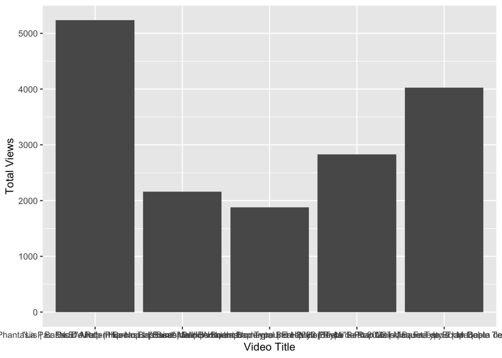
The goal is to practice data acquisition, data wrangling, and data visualization. I am using data from my Official YouTube Channel where I share my music.
The goal is to showcase visuals that are not on YouTube studio by default. While It took all this code to just show one visual -so far-, I am confident that with time I will add more to it.
I wanted to share this to remember my progress.
I am sure there is a lot to improve here. I welcome any feedback you have.
Here is the actual PDF export from R that looks much cleaner than what I shared here.
Feel free to download it for reference or to tailor it for your needs.
Until then,
Ernesto
 # Project and Contact Info -----
 # YouTube Exploratory Data Analysis (EDA), Data Wrangling and Visualization Exercises
 # A Portfolio Project By Ernesto Gonzales
 # Website: ernestogonzales.com
 # Email: hello@ernestogonzales.com

 # Background ----
 # I downloaded the all my YouTube Studio data from April 1st, 2007 to October 25th 2023
 # 3 Comma Separated Values (CSV)files where downloaded from my website
 # These files were sourced from my own YouTube channel metrics of all my videos

# Project Deliverables ----
 # To showcase a step by step process on Data Wrangling using dplyr and lubridate libraries
 # Showcase my steps on doing EDA by using Visualizations using ggplot2
 # Provide a final report using R Markdown to create both PDF files and PowerPoint reports

# 01. - Data Preparation and Data Wrangling ---- # 01.01 - Libraries Used----
library(tidyverse)
## ── Attaching core
## ✔ dplyr
## ✔ forcats
## ✔ ggplot2
## ✔ lubridate 1.9.3
## ✔ purrr 1.0.2
## ── Conflicts ────────────────────────────────────────── tidyverse_conflicts() ──
## ✖ dplyr::filter() masks stats::filter()
## ✖ dplyr::lag() masks stats::lag()
## i Use the conflicted package (<http://conflicted.r-lib.org/>) to force all conflicts to become errors
library(lubridate)

# 02. - Data Acquisition ----
# 02.2 - Initial Data Acquisition using read.csv command
table_data <- read.csv("~/Documents/00_Data_Projects/Content 2007-04-01_2023-10-26 Phantasiis/Table data.csv") chart_data <- read_csv("~/Documents/00_Data_Projects/Content 2007-04-01_2023-10-26 Phantasiis/Chart data.csv")
## Rows: 30260 Columns: 5
## ── Column specification ──────────────────────────────────────────────────────── ## Delimiter: ","
## chr (3): Content, Video title, Video publish time
## dbl (1): Views
## date (1): Date
##
## i Use `spec()` to retrieve the full column specification for this data.
## i Specify the column types or set `show_col_types = FALSE` to quiet this message.
chart_data
## # A tibble: 30,260 × 5
##    Date       Content     `Video title`               `Video publish time` Views
##    <date>     <chr>       <chr>                       <chr>                <dbl>
##  1 2007-04-01 6Etbk2iY2jA "\"Saint\" Melodic Boom Ba... Apr 27, 2022             0
##  2 2007-04-02 6Etbk2iY2jA "\"Saint\" Melodic Boom Ba... Apr 27, 2022             0
##  3 2007-04-03 6Etbk2iY2jA "\"Saint\" Melodic Boom Ba... Apr 27, 2022             0
##  4 2007-04-04 6Etbk2iY2jA "\"Saint\" Melodic Boom Ba... Apr 27, 2022             0
##  5 2007-04-05 6Etbk2iY2jA "\"Saint\" Melodic Boom Ba... Apr 27, 2022             0
##  6 2007-04-06 6Etbk2iY2jA "\"Saint\" Melodic Boom Ba... Apr 27, 2022             0
##  7 2007-04-07 6Etbk2iY2jA "\"Saint\" Melodic Boom Ba... Apr 27, 2022             0
##  8 2007-04-08 6Etbk2iY2jA "\"Saint\" Melodic Boom Ba... Apr 27, 2022             0
##  9 2007-04-09 6Etbk2iY2jA "\"Saint\" Melodic Boom Ba... Apr 27, 2022             0
## 10 2007-04-10 6Etbk2iY2jA "\"Saint\" Melodic Boom Ba... Apr 27, 2022             0
## # i 30,250 more rows
totals_data <- read_csv("~/Documents/00_Data_Projects/Content 2007-04-01_2023-10-26 Phantasiis/Totals.csv")
## Rows: 6052 Columns: 2
## ── Column specification ──────────────────────────────────────────────────────── ## Delimiter: ","
## dbl (1): Views
## date (1): Date
##
## i Use `spec()` to retrieve the full column specification for this data.
## i Specify the column types or set `show_col_types = FALSE` to quiet this message.
1.1.3
1.0.0
3.4.4
✔ readr ✔ stringr ✔ tibble ✔ tidyr
2.1.4
1.5.0
3.2.1
1.3.0
tidyverse packages ──────────────────────── tidyverse 2.0.0 ──
totals_data
## # A tibble: 6,052 × 2 ## Date Views ## <date> <dbl> ## 1 2007-04-01 0 ## 2 2007-04-02 0 ## 3 2007-04-03 0 ## 4 2007-04-04 0 ## 5 2007-04-05 0 ## 6 2007-04-06 0 ## 7 2007-04-07 0 ## 8 2007-04-08 0 ## 9 2007-04-09 0 ## 10 2007-04-10 0 ## # i 6,042 more rows

# Data Preview
table_data %>%
    glimpse() %>%
view()
## Rows: 393
## Columns: 7
## $ Content
## $ Video.title
## $ Video.publish.time
## $ Views
<chr> "Total", "VoitAdnwgnM", "D7PR8ezIUB...
<chr> "", "\"Esencia\" - Phantasiis | Bas...
<chr> "", "Oct 31, 2021", "Oct 29, 2021",...
<int> 91288, 5238, 4029, 2826, 2158, 1878...
<dbl> 2155.0593, 183.1138, 97.3285, 46.11...
<int> 687645, 36660, 23803, 47673, 15151,...
## $ Watch.time..hours.
## $ Impressions
## $ Impressions.click.through.rate.... <dbl> 6.39, 7.32, 9.58, 4.08, 6.06, 7.81,...
chart_data %>%
    glimpse() %>%
view()
## Rows: 30,260
## Columns: 5
## $ Date
## $ Content
<date> 2007-04-01, 2007-04-02, 2007-04-03, 2007-04-04, ...
<chr> "6Etbk2iY2jA", "6Etbk2iY2jA", "6Etbk2iY2jA", "6Et...
<chr> "\"Saint\" Melodic Boom Bap Type Beat 2022 | Pist...
## $ `Video title`
## $ `Video publish time` <chr> "Apr 27, 2022", "Apr 27, 2022", "Apr 27, 2022", "... ## $ Views <dbl>0,0,0,0,0,0,0,0,0,0,0,0,0,0,0,0,0...

# 03.00  - Initial Data Wrangling ----

# 03.01 - Table.csv -----

# Using pipes %>% with dyplyr commands to transform column names for legibility
# Used the mdy() command from lubridate in combination with mutate() function from dyplr
# To format the raw date in to MM-DD-YYYY time format for future analysis
table_data_wrangled_tbl <- table_data %>% mutate(video_published_time_clean = Video.publish.time %>% mdy()) %>%
mutate("Video ID"
       "Video Title"
= Content,
= Video.title,
= Impressions.click.through.rate....,
"ICR"
"Watchtime Hours" = Watch.time..hours.,
"Published Date"  = video_published_time_clean)

# After creating the new labels I used the select() command to isolate the new columns with proper names
# Created a new table that includes the new formatted date and new names
# It will be the basis for future analysis
table_wrangled_renamed <- table_data_wrangled_tbl %>% select(`Video ID`, `Video Title`, Impressions, ICR, Views,
`Watchtime Hours`, `Published Date`)

# 03.02 - Chart.csv ----

#chart_data %>% reframe(.by = Content, `Video title`, `Video publish time`,`Impressions click-through rate (%)`)
view(chart_data)
chart_data_wrangled <- chart_data %>% mutate(`Video publish time` %>% mdy()) %>%
    select(`Video publish time`, Content, `Video title`, `Video publish time`, Date, `Views`)
chart_data_wrangled %>%
    view()
# 03.03 - Totals.csv ----
totals_data %>%
    view()
# Data has the correct format
# A potential insight is to do a time series analysis based on the number of videos that got a CTR per 90 days

# 04. EDA using ggplot2 ----

#Initial Data Visualizations  -----
chart_data_wrangled
## # A tibble: 30,260 × 5
##    `Video publish time` Content
`Video title`
Date Views
## <chr>
## 1 Apr 27, 2022 ## 2 Apr 27, 2022 ## 3 Apr 27, 2022 ## 4 Apr 27, 2022 ## 5 Apr 27, 2022 ## 6 Apr 27, 2022 ## 7 Apr 27, 2022 ## 8 Apr 27, 2022 ## 9 Apr 27, 2022 ## 10 Apr 27, 2022 ## # i 30,250 more
<chr>
6Etbk2iY2jA "\"Saint\" Melodic Boom Ba... 2007-04-01     0
6Etbk2iY2jA "\"Saint\" Melodic Boom Ba... 2007-04-02     0
6Etbk2iY2jA "\"Saint\" Melodic Boom Ba... 2007-04-03     0
6Etbk2iY2jA "\"Saint\" Melodic Boom Ba... 2007-04-04     0
6Etbk2iY2jA "\"Saint\" Melodic Boom Ba... 2007-04-05     0
6Etbk2iY2jA "\"Saint\" Melodic Boom Ba... 2007-04-06     0
6Etbk2iY2jA "\"Saint\" Melodic Boom Ba... 2007-04-07     0
6Etbk2iY2jA "\"Saint\" Melodic Boom Ba... 2007-04-08     0
6Etbk2iY2jA "\"Saint\" Melodic Boom Ba... 2007-04-09     0
6Etbk2iY2jA "\"Saint\" Melodic Boom Ba... 2007-04-10     0
                   rows
glimpse(chart_data_wrangled)
## $ Content
## $ `Video title`
## $ Date
## $ Views
<chr> "6Etbk2iY2jA", "6Etbk2iY2jA", "6Etbk2iY2jA", "6Et... <chr> "\"Saint\" Melodic Boom Bap Type Beat 2022 | Pist... <date> 2007-04-01, 2007-04-02, 2007-04-03, 2007-04-04, ... <dbl>0,0,0,0,0,0,0,0,0,0,0,0,0,0,0,0,0...
<chr>
<date> <dbl>
## Rows: 30,260
## Columns: 5
## $ `Video publish time` <chr> "Apr 27, 2022", "Apr 27, 2022", "Apr 27, 2022", "...
chart_data_clean <- chart_data_wrangled %>% mutate("Video Published Date" = `Video publish time` %>% mdy()) %>%
    select(Content, `Video title`, `Video Published Date`, Date, Views)
chart_views_by_video_title <- reframe(chart_data_clean,.by = `Video title`, Views) %>% group_by(`Video title`)
total_views_by_video_title <- reframe(chart_views_by_video_title, `Video title`, Views)
total_views_sum_by_title <- total_views_by_video_title %>%
    group_by(`Video title`) %>%
    summarise(sum(Views))
Video_titles <- as.factor(total_views_sum_by_title$`Video title`) %>% bind_cols(total_views_sum_by_title$`sum(Vie
ws)`)
## New names:
## • `` -> `...1`
## • `` -> `...2`
viz_total_views <- ggplot(data = Video_titles, aes(`...1`,`...2`))
viz_total_views_labeled <- viz_total_views + geom_col(mapping = aes(`...1`, `...2`)) +
    scale_fill_brewer("Spectral", type = "seq", palette = 1, direction = 1) +
    labs( x = "Video Title", y = "Total Views")
viz_total_views_labeled